During my minor I attended an “Advanced Bioinformatics” course. For part of the exam each student was assigned a subset of samples from a GEO dataset to perform a RNA-seq differential expression analysis. This report uses samples from from Blanco-Melo et al., 2020 ¹ This analysis used the DESeq2 workflow by Love et al., 2014²

1 Introduction

To study the effect of SARS-COV2 on the transcription of genes A549 human cell lines were infected with USA-WA1/2020 SARS-COV2 virus or mock treated. The Illumina NextSeq 500 platform was used to sequence the cDNA library. The reads were aligned to the human reference genome (hg19) using a RNA-Seq Aligment App on Basespace. The resulting table containing the readcounts was uploaded to GEO and serves as a starting point for this analysis.

2 RNA-seq analysis

2.1 loading/installing packages

#install bioconductor if it's not installed yet.
if (!requireNamespace("BiocManager", quietly = TRUE))
    install.packages("BiocManager")
BiocManager::install(version = "3.12")

#install libraries if they are not installed yet
require("tidyverse") || utils::install.packages("tidyverse")
require("pheatmap") || utils::install.packages("pheatmap")
require("here") || utils::install.packages("here")
BiocManager::install("GEOquery")
BiocManager::install("DESeq2")
BiocManager::install("SummarizedExperiment")

#load libraries
library(tidyverse)
library(GEOquery)
library(DESeq2)
library(pheatmap)
library(here)
library(SummarizedExperiment)

2.2 Data downloading and organizing.

#Downloading expressionset and supplementary files from GEO.
GSE147507 <- getGEO('GSE147507', destdir=".", GSEMatrix = TRUE)
GSE147507_supp <- getGEOSuppFiles('GSE147507', makeDirectory = TRUE, baseDir = getwd(),
  fetch_files = TRUE, filter_regex = NULL)

#There is human and ferret data. We select the human data. 
gse_human <- GSE147507[[1]]

Organizing and manipulating the data to make it suitable for building a sumarizedexperiment object

# First we need to obtain the countsdata,phenodata,featuredata and metadata so they can be manipulated individually later.

#We start with assay data (countsdata)
raw_counts_human <- read_tsv(file = here::here("GSE147507", "GSE147507_RawReadCounts_Human.tsv.gz"))

#obtaining phenotypic data. contains all the info regarding each sample. 
phenodata_human <- pData(gse_human) %>% as_tibble

#First column of raw_counts contains te genenames (featuredata)
rowdata_human <- raw_counts_human$X1

# lastly we collect the metadata 
metadata <- experimentData(gse_human)

#Next we select the samples that the assignment calls for ("GSE147507: GSM4462336, GSM4462337, GSM4462338, GSM4462339, GSM4462340, GSM4462341)
coldata_human <- phenodata_human[21:26,]
assaydata_human <- as.matrix(raw_counts_human[,22:27])
rownames(assaydata_human) <- raw_counts_human$X1

#changing the colname to treatment to make more sense
colnames(coldata_human)[8] <- "treatment"

2.3 Generating a summarizedexperiment

#Now we make a summarizedexperiment 
se_human <- SummarizedExperiment(assays = assaydata_human,
                     rowData = rowdata_human,
                     colData = coldata_human)

metadata(se_human)$metadata <- metadata #adding metadata manually because the summarizedexperiment won't accept it.

# uncomment the next lines of code to inspect the assaydata, coldata and the metadata. 

#colData(se_human)
#metadata(se_human)
#head(assay(se_human))

2.4 Testing for differential expression using DESeq2

#differential expression analysis. The only variable that is changed between samples is treatment with SARS-CoV-2 or mock treatment. 

#make DESeq2 dataset
ddsSE_human <- DESeq2::DESeqDataSet(se_human, design =  ~treatment)

#filter all genes expressed less than 10 times.
keep <- rowSums(counts(ddsSE_human)) >= 10
ddsSE_human <- ddsSE_human[keep,]

#perform DESeq2 analysis
ddsDE_human <- DESeq(ddsSE_human)

2.5 Exploring the results

#getting the results of the analysis
res_human <- results(ddsDE_human)

#show top genes
res_human[order(res_human$padj), ] %>% head

## log2 fold change (MLE): treatment SARS.CoV.2.infected.A549.cells vs Mock.treated.A549.cells 
## Wald test p-value: treatment SARS.CoV.2.infected.A549.cells vs Mock.treated.A549.cells 
## DataFrame with 6 rows and 6 columns
##                  baseMean    log2FoldChange              lfcSE
##                 <numeric>         <numeric>          <numeric>
## STC2     3472.80474970729  4.01354416339484  0.101040911737679
## LAMC2    5759.15843475204  3.70298493699246  0.111152821502871
## GPX2     8870.37949591171 -2.78195864864618 0.0859738574901862
## C15orf48 2601.41563186467  2.74951039419932 0.0894554468106483
## FASN     6880.20205343698 -2.26011225041142 0.0751376739543801
## KRT8     41319.5434574062 -2.23441250828749 0.0773697350855379
##                       stat                pvalue                  padj
##                  <numeric>             <numeric>             <numeric>
## STC2      39.7219709756257                     0                     0
## LAMC2     33.3143584384568 2.39231057967507e-243 1.73406632367748e-239
## GPX2     -32.3581927094959 1.06402320224979e-229 5.14171478767173e-226
## C15orf48  30.7360869821516 1.87631215639893e-207 6.80022433282883e-204
## FASN     -30.0796142795643  8.9539490879128e-199 2.59610799854944e-195
## KRT8     -28.8796711765548  2.1495181208785e-183  5.1935940330626e-180

# show distribution of p-values
ggplot(as(res_human, "data.frame"), aes(x = pvalue)) +
  geom_histogram(binwidth = 0.05, fill = "#446e9b")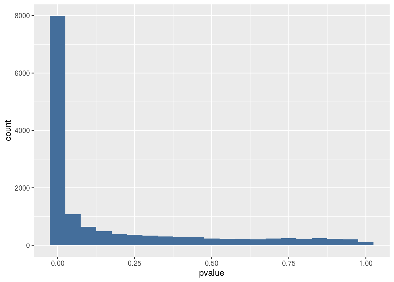

Histogram of p-values found in the results. Around 8000 genes have a p < 0.05 indicating they are differentially expressed. Looking at the background (p > 0.2) we can estimate that around 250 out of 8000 differentially expressed genes are false positives (3%).

#log fold change
#get resultnames to input into LFC function
resultsNames(ddsDE_human)

## [1] "Intercept"                                                          
## [2] "treatment_SARS.CoV.2.infected.A549.cells_vs_Mock.treated.A549.cells"

#apply Log 2 fold change
resLFC_human <- lfcShrink(ddsDE_human, coef="treatment_SARS.CoV.2.infected.A549.cells_vs_Mock.treated.A549.cells", type="apeglm")

#make a vulcan plot
DESeq2::plotMA(resLFC_human, ylim=c(-2,2))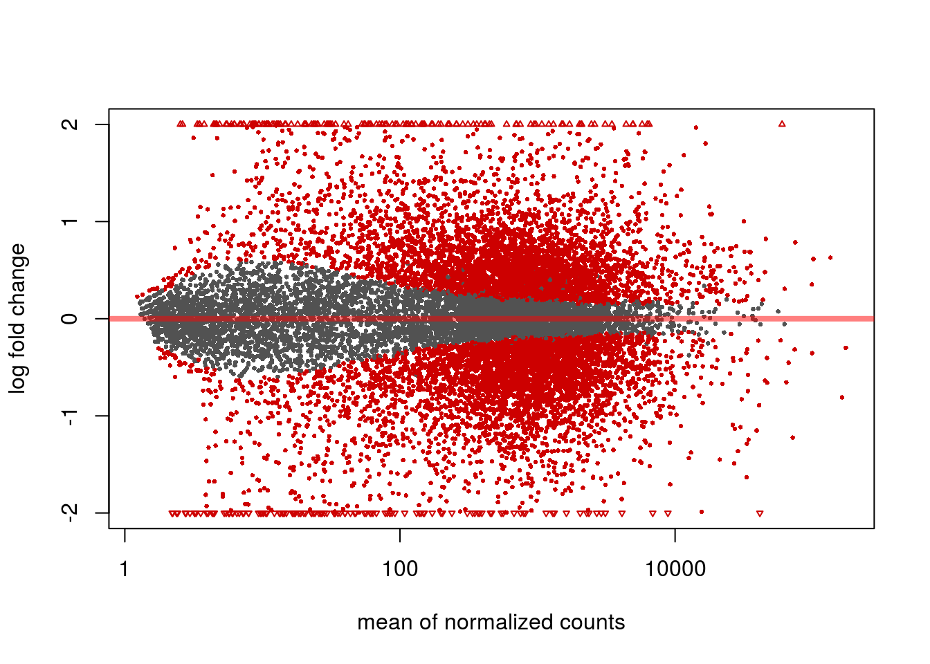

MA plot. Blue dots represent differentially expressed genes

#principal component analysis
ddsDE_rlog_human <- ddsDE_human %>%
  rlogTransformation() 


ddsDE_rlog_human %>%
  DESeq2::plotPCA(intgroup = c("treatment")) +
  geom_vline(xintercept = 0, linetype = "dashed", colour = "red") +
  geom_hline(yintercept = 0, linetype = "dashed", colour = "red")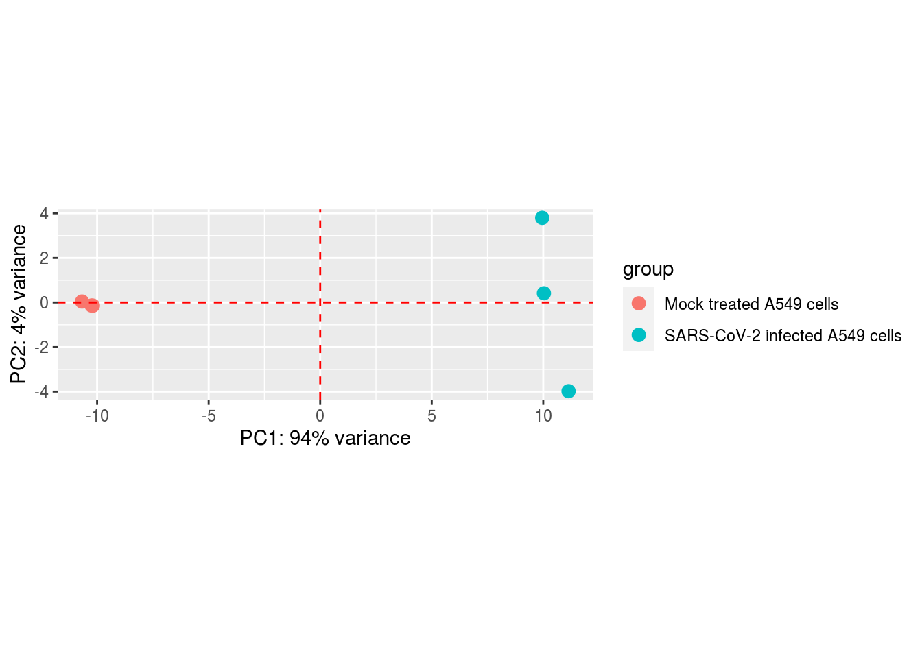

Principal component analysis shows the biggest variance in the data is between treated and mock treated cells (as is to be expected). There is also variance between treated cells but this only accounts for 4% of the variance in the data. The mock treated cells don’t show much variance between themselves.

2.6 Heatmap

matrix_results <- assay(ddsDE_rlog_human)

ind <- matrix_results %>%
  rowMeans() %>%
  order(decreasing = TRUE) 

top20 <- matrix_results[ind[1:20],]
heatmap <- pheatmap(top20,
                    scale = "row")
heatmap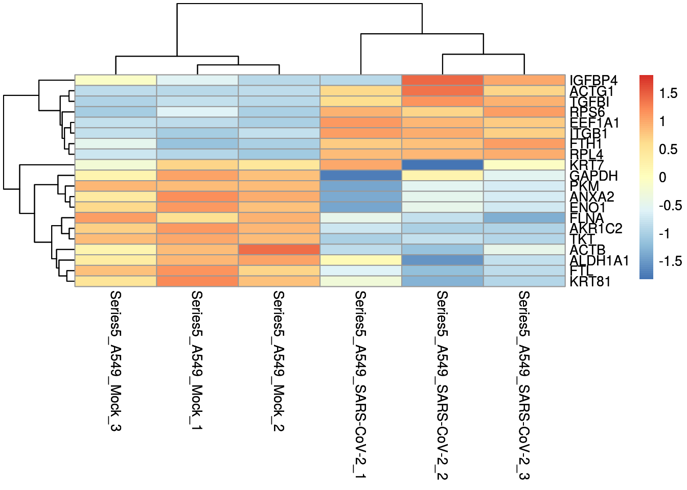

Heatmap clustering of top 20 of up and down regulated genes.

3 Conclusion

Alot of genes in the A549 cells get up or down regulated when infected with the virus. analyzing what pathways are associated with the differentially expressed genes belong to.

4 Bibliography

Daniel Blanco-Melo et al., “Imbalanced Host Response to SARS-CoV-2 Drives Development of COVID-19,” Cell 181, no. 5 (May 2020): 1036-1045.e9, https://doi.org/10.1016/j.cell.2020.04.026.↩
Love, M.I., Huber, W. & Anders, S. Moderated estimation of fold change and dispersion for RNA-seq data with DESeq2. Genome Biol 15, 550 (2014). https://doi.org/10.1186/s13059-014-0550-8 ↩

RNA-seq: SARS-CoV-2

Thomas Baardemans

22-6-2020